Receiver Design

Now I've shown the front end of the radio it's time to look at how the signals it selects will be demodulated and the time code extracted. Actually, the demodulated signal is fed back into the front end of the receiver and used as an AGC control. This was seen in outline back on the page where the small signal amplifier simulation was described. There I just created the quickest possible simulation model with the required functionality. Using ideal diodes and capacitors is relatively easy. Real components just aren't that good.

The back end of the radio actually breaks down into four discrete modules;

• An instrumentation amplifier converts the differential signal from the front end into a single ended signal.
• A detector converts the sine wave from the front end, into a signal whose average value is non zero.
• Then, an integrator averages the signal into a DC value which is proportional to the magnitude of the received signal at the antenna.
• Finally a scaling amplifier, allows the average value to be magnified or reduced prior to reuse as an AGC signal.

This outlines the functionality which was simulated previously.

The Usual Suspects

In addition to functions simulated previously, the last two modules have additional capability which allow a demodulated time signal to be taken from the cicuit as an open collector output suitable for connection to a microprocessor such as the ubiquitous MSP430, AVR, or PIC. Actually you can connect this receiver almost directly to any UART, and later I'll outline a circult for doing RS232 level translation using the same transistors and op-amps I've used everywhere else on the radio. I'll include the C source I used on my PC too.

To demodulate the signal for conversion into an actual digital time signal, the integrator has a second averaging path with it's own, separate, integration time. The existing averaging path, previously discusssed is considered to be the slow integrating path. The slow path converts the detected sine wave into a DC voltage with a time constant of perhaps 3 seconds. Such a time constant is consistent with ensuring the AGC loop is slow and stable. If the AGC loop time is too fast, with such a wide dynamic range as we have, the whole radio could become quite unstable.

Receiver Behaviour

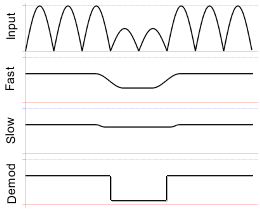
The slow path is augmented with a fast averaging/integrating path. The time constant of the fast path is about 3.2 milliseconds. This is obviously about 1000 times faster. In principle, it is fast enough that it indicates the incident signal power more or less instantaneously; but not so fast that the individual radio frequency cycles can be seen.

When combined in a comparator with hysteresis, the fast and slow averages reveal changes in amplitude of the transmitted signal. The transmitted signal is Continuous Wave with 100 per cent modulation. It is arranged at the transmitter, and in the digital data protocol, that the transmitter be transmitting most of the time. Short periods where the transmitter is "off" cause the short average voltage to fall quickly, but the long average cannot immediately follow. This difference in the short and long averages can be used to "receive" the signal. You can see a graphical outline of this process in the diagram to the left.

Particular care is taken to buffer signals either side of the integrating capacitors. It is important that preceeding and subsequent curcuit dynamic behaviours cannot affect the time constants in the capacitors. I'll visit this aspect in detail shortly.

Instrumentation amplifier

Detector

This, our first of three devices could be as simple as a diode. Its function is to convert the incoming signal from a sinusoid into something that can be averaged, and measured.

In essence it's the RMS problem. Typically if one wants to measure the magnitude of a sine wave, the signal would vary with time. One can never accurately say that the signal size is five volts peak to peak because instantaneously the signal would be some other intermediate value. Even if one measures the envelope of the signal over a time period greater than the signal cycle time, the envelope can vary from cycle to cycle. If compressed, the peak to peak value of the now pseudo-sine function no longer represents the energy in the signal.

Root of Mean Squares

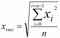
Mathematically a sinewave can be averaged by squaring the samples prior to averaging them. The square function rectifies because any number multiplied by its-self is positive. After the averaging, a square root of the result is taken to normalise the numeric value and to give relative meaning. This is the Root of Mean Squares.

The signal is a sine function and its average value is zero. We could square the signal value electronically, but we don't need to. All we need to do is recognise that that the signal must be modified in a consistent way to allow averaging. If the negative trending half of the sine cycle is removed, then an average value can be found in just the same way as with the square function. The basic implementation of a detector is a rectifier or diode, which simply cuts the negative trending part of the signal and allows averaging.

In this implementation, I used a precision full wave rectifier. It really doesn't have to be this complex at all. Certainly use of a simpler circuit would change the measured average, but actually that's not too important. What we're really interested in is how the average changes with time. The AGC circuit will be sensitive to the actual average value we ultimately measure. Since we'll be programming the gain of the AGC loop on a potentiometer it doesn't actually matter. The main thing about the precision full wave rectifier is that it is an interesting circuit. It's actually quite rarely used as implemented in Op-Amps. In a natural way the approach seems more suitable even than the squaring method used in RMS calculations. The absolute value circuit changes the sign of the negative going part of the signal. This is exactly what we want because we can change the sign without squaring, even if that is more than we really need!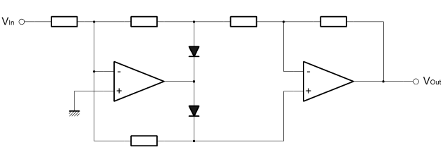

The circuit above is the absolute value circuit used. I've not described it here, because there is a whole page dedicated to it elswhere on the site.