Filter Simulation

Having looked at the basic scheme for introducing selectivity into the receiver, it's really time to look at how the details pan out. I've described that we'll be using a basic tank circuit to short out the unwanted signals from the antenna.

The diagram below shows how we'll realise the basic tank circuit that we're using to select the 60kHz MSF radio signal;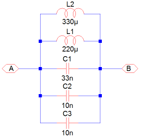

The circuit has been designed around preferred component values. The capacitors used are simply the small ceramic capacitors that are widely available. The range for selection of these components is simply huge. High precision components are easily obtained, and for this reason is seems crazy not to take advantage. It would be possible to use a home made inductor, and a variable capacitor, but it seems prudent not to throw away such precision where it is so cheap and readily available.

The variable slug allows considerable tuning of the inductance value. To give an idea, the 220uH inductor can probably be varied in the range 150uH to perhaps 300uH. In the form that we have the tank circuit we'll have two such inductors in parallel, and although the range is reduced, it is still satisfactory.

The diagram below shows the test harness for the cascaded filter and amplifier arrangement. The amplifier is the same as that developed on previous pages. This time the AGC port of each amplifier has been set to cause maximum gain in each amplifier. This gives us an indication of the best possible performance of the front end. You'll notice that the filter above has simply been connected directly between the balanced lines. The tank won't work without, at least, a source and load impedance. It's not perfectly true, but the amplifier inputs are assumed to be infinite impedance. The output impedance of the amplifier stages are assumed to be the all important source impedances. The amplifiers develop a voltage in their load resistors, as a result of the signal. In theory this is the voltage we measure at the amplifier inputs.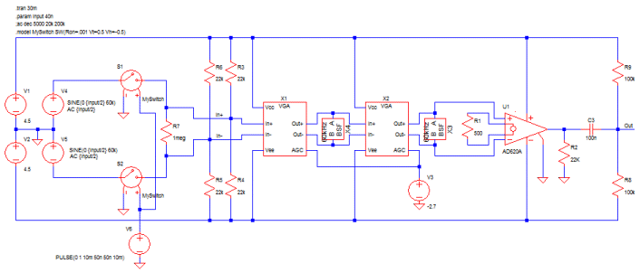

You'll notice that the input circuit for the test harness has a couple of switches and a 1M ohm shunt resistor, across the input. The switches are connected to, and controlled by, a pulse generator. This allows us to modulate the input signal, and consequently look at the envelope rise and fall times - much like we did with the regenerative amplifier on the previous page. The 1M ohm resistor is needed by the simulator. The switch is fast, and it generates an unwanted spike, which leaves to the simulator struggling to do the sums. It can be more or less ignored since it is part of the harness and not the test. It just smoothes the simulation along.

The other thing you'll notice is the use of the AD620 on the output. The AD620 is an instrumentation amplifier. It is really designed for a precise gain, in instrumentaion applications. Typically it is the first amplifier in a bridge measurement circuit, perhaps like strain guage or a temperature bridge. Such signals would be typically small, and need precise measurement. Here, we're using it to receive small signals. I happen to have a few lying around, so that drove the choice, there are probably more suitable choices, but the AD620 is a nice amplifier.

Importantly a standard op-amp is not a good choice in this particular situation. The AD620 has very low input offsets for a linear amplifier. It can be thought of as three standard operational amplifiers. This is important because it allows the input impedance of each input to be as high as possible. Two "first stage" amplifers are configured as non-inverting amplifiers, or at least the input circuits look that way. Since there is no other connection to each input node, the input impedance is as high as possible. Gain is set to 100, by the 500 ohm programming resistor.

This amplifer is the one we'll use in the final design to go from the balanced format, to single ended. It is where, finally we can begin to use op-amps for working on the RF signal. Here I've just used it as a convenient way to combine the balanced line so we can see a reasonable indication of the real performance of the filters, in circuit.

As I mentioned earlier, the selectivity that we achieve in the tank circuit is hugely dependent on the load impedance. The higher we can make the load impedance and the smaller the source impedance, the better selectivity we will achieve. In practice the first filter in the chain will give poorer performance than the second. The AD620 has a higer input impedance, than our home brew amplifiers. Sadly, the AD620 cannot deal with signals as small as those we expect from the antenna. For this reason we can accept the differences in performance between the two filters.

In any case, it doesn't matter. We'll be looking at the combined performance of both filters. In fact, the diagram below shows the frequency response for a 40nV input signal at the output of the AD620;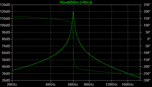

You can see that the selectivity is more or less satisfactory. The signal size, on resonance is about 120dBV, which equates to just about 60mV, from our input of 80nV, which is a voltage gain of about 8.25 million, including the filters and any losses. You can't see it so easily from the graph, but I can say that if one zooms in, the 3dB bandwidth is about 600Hz. Originally we wanted 500Hz in the spec, but 600 is satisfactory. We already saw how we could improve this on the previous page. Going the extra mile probably isn't worth the extra components. We're building this receiver to find out what we might need to do. We could perhaps design space onto the circuit board for an additional filter stage. It won't make sense to put additional transistors on, because they are difficult to link out in the likely event that we don't use them. The filter can be placed on the board but the components not fitted. If we do need another cascaded amplifier stage we can build it quickly on stripboard and attach it on the front of the receiver. In that case we could then fit the filter network and see improved selectivity.

Broadly speaking the overall frequency response here is consistent with the dynamic range specs we originally set out. Although the dynamic range is not related to the large scale "depth" of the filter, we can see that broadly the 60dB dynamic range from the spec is consistent with the depth.

In the time domain the amplifier / filter is perhaps not as good as we would like. With envelope risetimes of two or three milliseconds, we're certainly into the realm of the "tail" we witnessed on the regenerative amplifier. It's not ideal, but the benefit is seen in the selectivity of the filter. If we were to reduce the input impedance of the amplifiers, with a shunt resistor, we could shorten the envelope risetimes. As it is we have good selectivity, and such a shunt resistor, would cause that performance to deteriorate.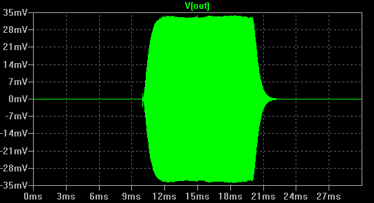

Had we used regeneration as well as this filtering scheme, we could have expected a significantly greater "tail". That's par for the course. Without it, the envelope rise / fall times, are in the order of one or two milliseconds. This will have a small impact on the absolute instantaneous measurent of MSF time. In general terms thats one or two thousandths of a second, which isn't much. It has to be remembered that there will be a similar effect due to the propagation time of the radio waves. Our delay is greater, but it's still nothing like noticable for a basic solution like ours. Most importantly though, there is no detimental effect on the spacing of individual seconds. Though there is a small time delay in signalling, the envelope risetimes affect all edges the same. In an integral sense the time tracks well.

In general it seems the selectivity is looking fairly good, especially by comparison with our regenerative solution. That solution had a similar enevelope risetime, but only a 1kHz 3dB bandwidth. Broadly I think we can be fairly happy with the filter performance, even though it is really quite a basic scheme.

Since we've seen how the AD620 will bring the balanced signals together, we can now work with op-amps. So far I've covered my thinking in some degree of detail. I think that people are much more familiar with the use of op-amps and single ended signals, so I won't dwell in quite the same way on the remaining circuit functionality. On the next page will cover the remaining aspects of the receiver.