Filter Design

We've looked at how we're going to produce the basic gain block. With a little imagination it's possible to see that the gain block we tested previously could be used either as a variable gain block or as a fixed gain block. Now we have these two elements, we have to think about how we can introduce selectivity into the front end of the receiver.

Overview

Traditional Tuned Amplifier

I was originally thinking along the lines of the traditional approach to the design of a TRF which would typically use a tuned circuit in the collector circuit of an amplifying transistor. I'd also observed the more complex (perhaps) structures of single chip MSF receivers, where a quartz crystal is used as regenerative crystal filter.

From the perspective of our small receiver, niether approach is particularly attractive. I've been attempting throughout to avoid regeneration, because it has a tendency to "mush" the signal. We'll look at this shortly. Regeneration works by feeding back some of the amplified signal into the input of the receiver. It's really very effective at making a small signal, much larger, as I'm sure you can see. The problem with it, is that it has a time delay associated with it. For any given input signal, it takes some time for the regeneration to stabilise.

Regenerative Tuned Amplifier

Since we're building a timecode receiver, we're really looking to minimise any phase artifacts. In practice these are going to be most signifcantly generated by atmospheric multipath effects. We can't do anything about the atmospheric effects, but still it seems prudent to avoid regeneration if we can.

For the single chip solutions regeneration becomes much more attractive, because the use of a crystal means that a single external component can be used to set the frequency of reception, and with a supremely exaggerated Q factor. This is important because it is quite difficult to impement big capacitors and inductors on a semiconductor wafer, and the use of multiple external components increases the all important pin count.

Since we have no such wafer limitations; I discarded the quartz crystal idea, but when I thought about the traditional tuned amplifier, I had some more reservations. The problem is that to implement such a solution we would need to find a centre tapped transformer. The transformer would need to have with a particular inductance so that we could then use a variable capacitor to form a tank circuit.

A variable centre tapped transformer is an unlikely component, and a complimentary selection of variable capacitors are themselves not easy to find. Not only is the transformer a difficult component to obtain, it's also quite bulky and because of our long tail pair small signal amplifier design, we'd need two such transformers for each amplifier stage. Finally this type of circuit violates our originally stated desire to avoid variable capacitors.

Differential Tuned Amplifier

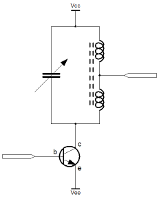
As I thought about this problem I realised that it would be possible to implement a simple and highly effective solution, just because we've already elected to amplify the small signal in a balanced way. By connecting a simple tank circuit between the balanced lines we can cancel the magnitude of frequencies that are not resonant. Those that those that are resonant, remain unaffected.

Implementing a solution this way means that we only have to find single inductors of suitable value. Such an inductor is far easier to obtain, in a wide range of values. In addition, single value inductors can be obtained in a form with a movable "slug" which affords tuning of the inductance. Overall the solution is quite scalable and represents a filtering scheme which is (more or less) independent of the rest of the design.

Closer inspection of regeneration

It may seem that I've summarily discarded the idea of regeneration, so I felt it important to look at why this is. The circuit below depicts a SPICE simulation of a regenerative amplifier, using a crystal as the frequency selective element. I honestly don't know if one would find this in a book, I just bashed it out using idealised components in SPICE. I'm not entirely happy that the design has been simplified to the best possible extent, but it seems to work. Importantly it demonstrates the problem that I'd originally imagined with regeneration.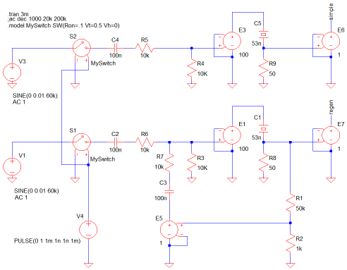

In the diagram there are essentially two circuits. The top and bottom circuits are identical but the lower circuit has positive feedback for the purpose of regeneration. By drawing the two circuits like this, we can directly compare their performance and see the effect of regeneration in the simulator.

LtSPICE doesn't have a specific model for a quartz crystal. Most of the standard linear components have a the capacity to specify user parameters for parasitic inductance and resistance. What I've done is model a crystal around a series inductor and capacitor. It's not strictly correct for a crystal, but in this example we're not looking at the properties of the crystal. What we're interested in is the regenerative action.

Both circuits have identical stimulae. In this case it's a 60kHz oscillator and a voltage controlled switch. The switch is nominally on for a 1ms period in the middle of a 3ms transient analysis simulation. In a second I'll show the transient simulation, but I also did an AC analysis, and I'll put that up too.

You can see from the lower (regenerative) circuit that the output from the amplifier (shown with voltage gain 100) is fed into the crystal, and then into an output buffer. Some proportion of the unbuffered output is taken off, buffered again and fed back into the summing junction on the input. Since the amplifiers are ideal, they have infinite input resistance. I've replicated part of the summing junction on the circuit at the top (simple) so that the overall gain should be, more or less, identical.

Since the regeneration is positive feedback, we obviously have to be careful that the signal fed back into the input of the amplifier, is not greater than unity. If we feed back a proportion of the output whuich is greater than the input which caused the output, then the amplifier will quickly saturate. All the time that the feedback is less than unity, the feeback loop will merely have the effect of multiplying the gain.

The simulation waveform below shows the transient (time domain) analysis of the regenerative circuit.;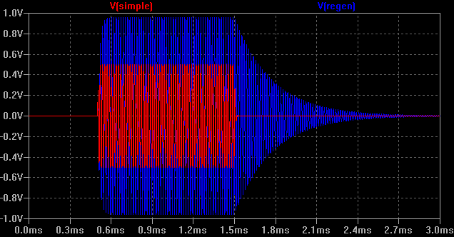

As you can see in the simulation the envelope risetime is more or less comaprable between the two circuits. The regeneration has allowed us to double the signal size, In contrast however, the regenerative circuit has a significant "tail". As the input signal is applied, the output signal rises with it, obviously dependent on the characteristic of the filter. This element could be eliminated by correct matching of the filter to the source and load impedances.

In our case the frequency is low enough that such matching is not critically important, and we could do without the effect of minimising "insertion losses" on "voltage gain". The notable feature is the "tail". This is not, in the main, due to the filter, but the regeneration. Certainly it is true that as the Q of the filter improves, the envelope can change in this way, but normally that would be similar on both the rising and falling edges of the envelope.

Here, it is clear to see how the regenerative effect, in conjunction, with the filter maintain oscillation in the circuit, long after the stimulus has gone. This is a typical "mush effect". What is happening, is that the signal has gone but the energy remaining in the filter, is enough to multiply through the regeneration and prolong the decay. By proper matching, the effect can be reduced, but then one needs more regeneration to achieve similar voltage gain.

Although the regenerative action has side effects, it also has some benefits. The next diagram shows an AC analysis or frequency sweep of both circuits. The additional gain, has the effect of bringing the pole much closer to the axis. This, perhaps, is obvious but I'm not sure it's intuitive. Overall we've got an additional 3dB of gain, but we now have some 30dB of additional selectivity (nominal). When thinking about the pole, it is clear that this is simply due to the hyperbolic nature of the plane.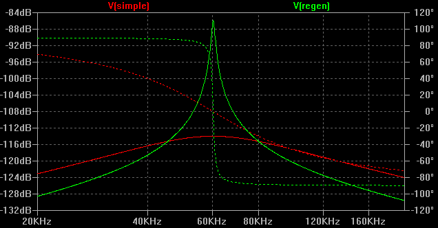

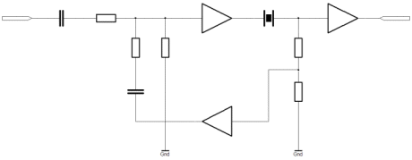
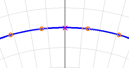
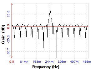
As you can see the filter has gone from being, a bit on the flat side, to being relatively useful. Let me be clear, there is plenty of potential for improvement and optimisation here, but we've now seen the basic problem. It's always reasonably difficult to make a regenerative circuit behave correctly. It can have significant benefits on reducing circuit complexity, and improve both sensitivity and selectivity. The problem, however, is that it can become difficult to maintain stability, and there are time domain penalty effects on the signal.

In our particular case, the MSF signal is defined by it's second marker. In practice this is the falling edge of the RF envelope at the beginning of each second. To indicate the instant of a second beginning, the transmitter is switched off for 100ms. At the instant the signal begins to fall, the second is deemed to have begun. As you can see, the idea that regeneration might selectively introduce a "tail" on such a falling edge is not appealing. As we may yet see, these envelope rise / fall times may simply become a static feature of achieving the required level of sensitivity and selectivity. The thing with regeneration, is that it focusses a problem exactly where we don't want one.

Cascaded filter sections

Having decided to use a simple filter, we must begin to think in more detail about the actual filter section that we implement. Some considerable thought went into this. Although I've already proposed the solution we will ultimately adopt, it seems important to think about the passive alternatives that I discarded.

In general terms we've come to a solution that uses passive filtering. It's not until we reached that answer, that we begin to think in more formal terms about the types of filter we could choose. Nothing has been said about active filters, for example. The truth here is that we could, perhaps, think about active filters in terms of the frequency requirements that we have, since the 60kHz carrier is a fairly low frequency. We already plan to use op-amps as the active element later in the signal path. The trouble really is the signal size. We're already using transistor amplifiers because the signal is so small. We really need lots of gain to get "high Q" or good selectivity, as we saw in the regenerative example. Even at 60kHz this is problematic with op-amps.

Perhaps we could do all of our filtering after the signal is big enough to work with in an op-amp? This too is impractical. We already looked at AGC and concluded that the gain control was best located at the front of the receiver. The same is true for the selectivity, for similar reasons. Without the selectivity, in the front end, an unwanted signal anywhere in the band could saturate the receiver, and then we're unable to receive the particular frequency we want.

Really, unless we build our own amplifiers, which leads to higher component counts, active filtering is out. That is to say filters that use frequency selective components in the feedback loop of an integrated circuit differential amplifier. In any case the nyquist stability requirements of such schemes become impossible to manage as frequency rises. Active filters are a superb solution for low frequency applications. Cascaded passive filters make much more sense as the frequency rises.

I did look at a variety of ad-hoc canonical approaches using the basic tank circuit to build an arbitrary response, using both poles and zeros. One can achieve surprising results this way, as the diagrams below show. Magnitude responses can be made superb for our application, especially since we actually want just a single pole at our frequency of interest.

In the first example, which I partially developed through into spice, you can see the broad mechanism used. By pacing a single pole at the frequency of interest, one can then flatten out the rest of the band with carefully placed zeros.

Pole Zero Plot	Magnitude Plot

I only partially developed this in spice, because it was already too big, in terms of component count. You can see how using such techniques we can achieve some tremendously powerful filters. Here we achieved a 3dB bandwidth of 175Hz, but we could easily have done better by moving the first zeros inwards. Irrespective you can see how it is possible to work in this way;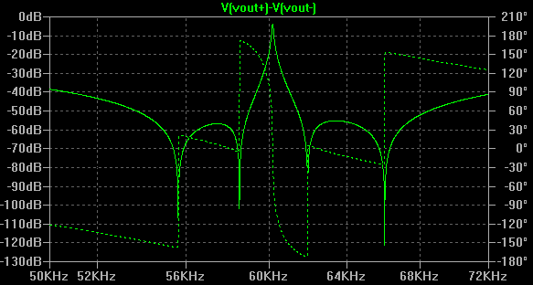

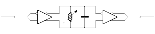
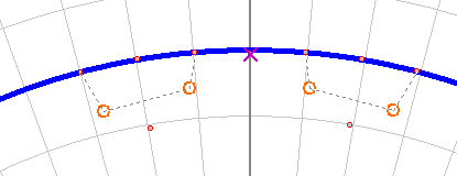
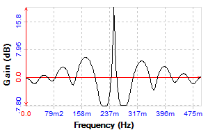
Looking at this, I thought it might be worth reducing the number of zeros, in an attempt to bring the component count down. This final alternative brings the component down considerably. The first (partially simulated) filter here used fourteen zeros and gives neary 50dB's of selectivity. The filter below, used ten zeros, and only achieved 15dB's of selectivity - but it wasn't trying as hard!

Pole Zero Plot	Magnitude Plot

It must be bourne in mind that each pole or zero needs a minimum of two components, and that to make the filter realisable, one may have to place poles on top of one another. Perhaps attenuation of the signal becomes too great in the filter as sections are cascaded. There is a practical limit to the complexity that is desirable. Personally, it is my belief complex filters like these do have a place, but that the place is mainly in the digital domain. There, digital multipliers have controllable precision, and can be re-used. Unlike the passive components, which interact when stages are cascaded, in the digital domain the equivalent to a capacitor or an inductor - the multiplier - can be reused for more than one pole or zero.

For the purposes of our small radio, the simple tank circuit will suffice. It's probably a bit of a cheat when compared with a well designed properly matched "m-derived" filter. Nevertheless, the power of just a couple of components to give a huge amount of selectivity is so attractive, one just has to stand aside from the issues of formality and conclude that it's the right way.

On the next page, we'll take the basic differential amplifier / filter, and cascade it so that we can begin to see the kind of sensitivity and selectivity we can achieve.